Understanding Stacked Column Charts
A stacked column or bar chart is similar to a basic vertical bar graph, except the bars are divided into colored segments representing different subgroups or categories. These categories are “stacked” on top of each other vertically to show their contribution to the whole column, which represents the aggregate total.
The key advantage of a stacked chart is it allows the viewer to immediately discern both individual and cumulative percentages or amounts in an intuitive format. Studying the segments makes it simple to spot the largest or smallest categories. We can also quickly analyze trends by subgroup within the same overall variable.
Situations where stacked column charts shine include:
- Comparing sub-category amounts to overall totals
- Tracking multiple time-based elements as a sum total
- Viewing market or demographic breakdowns
- Financial reporting and analysis
- Preparing your data
Before we begin building visualizations, it’s critical to have clean, well-organized source data. Our sample dataset tracks quarterly sales performance by product line—but this could easily be adapted for other needs.
The most essential step is structuring our spreadsheet to have one column for the primary category we want to graph (in this case, each quarter), and subsequent columns for the sub-categories (product lines) that will form each stacked element.
Example Structure
This shows the quarterly costs broken down into office categories.
| Quarter |
Furniture |
Office Supplies |
Technology |
Total |
| Q1 |
$10,000 |
$5,000 |
$15,000 |
$30,000 |
| Q2 |
$8,000 |
$6,000 |
$12,000 |
$26,000 |
| Q3 |
$12,000 |
$7,000 |
$10,000 |
$29,000 |
| Q4 |
$11,000 |
$8,000 |
$13,000 |
$32,000 |
With clean, well-formatted source data, we can start visualizing!
Step-by-Step Process to Creating a Stacked Column Chart in Excel
Many popular spreadsheet and data analysis programs allow users to generate stacked column or bar charts. The exact steps may vary slightly across platforms, but our example uses Excel due to its widespread adoption.
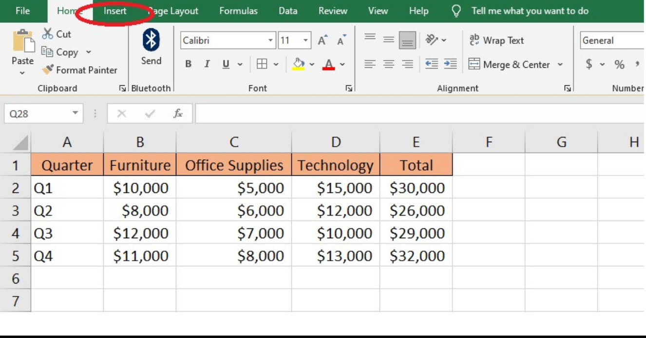
1. Create dataset in Excel and Click the Insert tab.
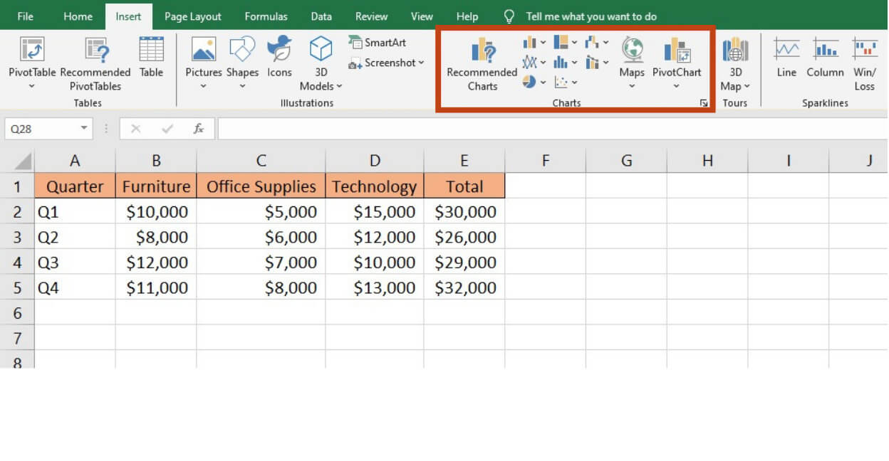
Within Excel, click the Insert tab on the command ribbon and select the Column chart option under Charts. This will insert a basic 2D column chart drawing from your existing data table.
2. Navigate to the “Charts” section and choose Stacked Column Chart
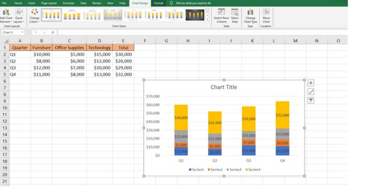
To convert the basic columns into a stacked format, find Chart Elements within the Chart Design tab. Click the dropdown arrow underneath this and hover over Change Chart Type. Here you will see options for Stacked Column Chart or 100% Stacked Column Chart.
The only difference is that 100% stacked columns adjust scale to always fill each column completely from bottom to top. Pick your preferred style for the use case.
3. Customize colors, labels, axes, and more
Now the column segments should be layered to illustrate contribution to the quarterly totals! From here, we can customize colors, labels, axes scales, and more to tailor the chart.