Understanding CONCATENATE
The CONCATENATE function in Excel is a tool for combining texts from multiple cells into a single cell. The function is essential for creating unique identifiers, merging client data, or generating comprehensive reports.
The syntax for CONCATENATE is:
=CONCATENATE(text1, [text2], …)
Here, “text1” represents the first item to be merged, while “[text2]” and any subsequent arguments are optional additional items.
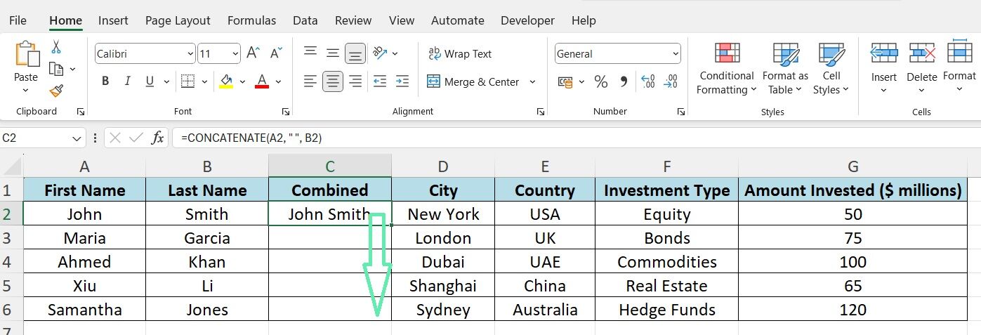
Let’s consider a practical example using our investment banking dataset. Suppose you combine investors’ first and last names for more transparent financial documentation.
You can do so by using the following formula:
=CONCATENATE(A2, ” “, B2)

In the above example, A2 contains the first name, B2 contains the last name, and the space in quotes (” “) adds a separator between the two. By dragging the formula down the column, you can quickly merge the names of all investors in your dataset.


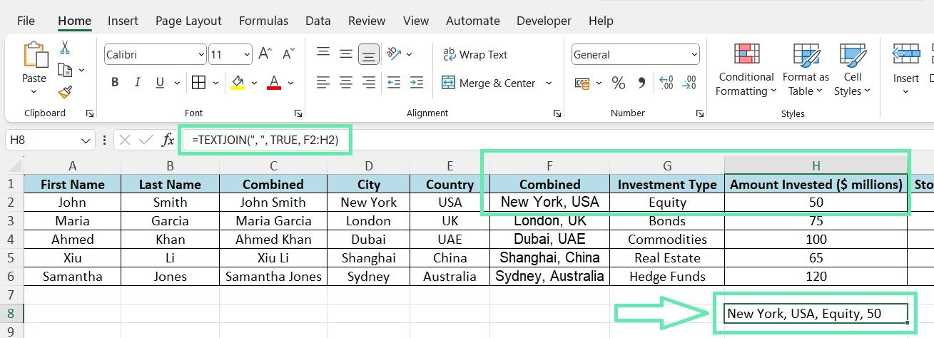
Another everyday use case in finance is merging city and country information to view client locations comprehensively. Assuming the city is in column D and the country in column E, you can use CONCATENATE as follows:
=CONCATENATE(D2, “, “, E2)

The above formula combines the city and country with a comma and space separator, resulting in a merged location format such as “New York, USA.”
Exploring TEXTJOIN
Although CONCATENATE is a valuable function, it may come with limitations when working with complex merging scenarios. Luckily, Excel 2019 introduced the TEXTJOIN function, which allows for concatenating text strings with a specified delimiter and the option to ignore empty cells.
The syntax for TEXTJOIN is as follows:
=TEXTJOIN(delimiter, ignore_empty, text1, [text2], …)
Where:
- The ‘delimiter‘ argument specifies the character or string between each merged item. For example, a comma as the delimiter will separate each item with a comma.
- The ‘ignore_empty‘ argument decides if empty cells should be included in the merged result (TRUE/FALSE).
- If set to TRUE, empty cells will be skipped.
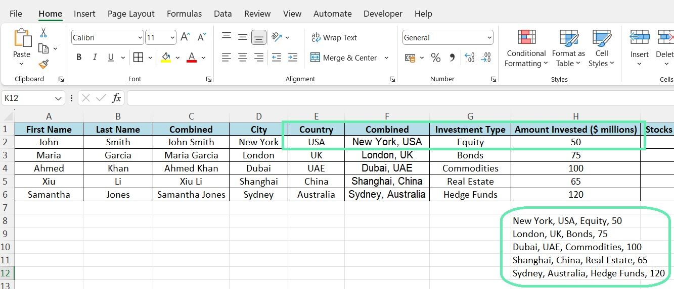
Let’s explore a practical example using our investment banking dataset. Create a formatted list of investment types for a client using columns F-J; some cells may be empty.
You can use TEXTJOIN to create a consolidated list as follows:
=TEXTJOIN(“, “, TRUE, F2:H2)

The formula sets the delimiter to comma and space and skips empty cells to display a formatted list of investment types.

Combining investment amounts with their corresponding types can be quickly done using the TEXTJOIN function. Assuming the investment amounts are in columns H through K, you can use the following formula:
=TEXTJOIN(“, “, TRUE, “Amount Invested: $” & SUM(H:H), “Stocks: $” & SUM(I:I), “Bonds: $” & SUM(J:J), “Mutual Funds: $” & SUM(K:K))

The above formula concatenates each investment type with its corresponding amount, separated by a colon and a dollar sign. The result will provide a clear overview of the client’s investment allocations:
- Amount Invested: $410
- Stocks: $100
- Bonds: $72
- Mutual Funds: $160
Download Excel Template


