Adding Compound Annual Growth Rate (CAGR) to Excel Charts

As an analyst or investor, being able to quantify and compare growth rates is critical to financial modeling. Among the key metrics to assess growth is the Compound Annual Growth Rate (CAGR). CAGR boils down a company or investment’s uneven growth path into a smooth, annualized rate. It factors in the compounding effect over time.

In this guide, we’ll unpack everything you need to know to understand CAGR:

• CAGR Definition & Use Cases
• Calculate CAGR in Excel
• Excel Shortcuts
• Visualizing CAGR on Excel charts

We’ll show you how to calculate CAGR in natively through Excel, provide a few shortcuts and show you how to add CAGR to charts.

Let’s start with an intro of CAGR: “what is it and why is it important?”

CAGR: Definition and Why it Matters?

As previously mentioned, Compound Annual Growth Rate measures the annualized growth rate of an investment over a specific time period with compounding returns. An example of this could be, if a stock grew from $10 to $20 over 5 years, its compounded annual growth rate would be 14.8%. Extrapolating that 14.8% out over the next 5 years, we’d see $40 a share.

Some other ways CAGR can be used:

• Volatility: It smooths out volatility in returns and provides an easily understandable growth metric. Unlike average returns, CAGR factors in compound growth.
• Comparisons: CAGR allows comparisons of growth rates across different time periods. You can compare the 3-year CAGR to the 5-year CAGR for example. You can also create quarterly and monthly growth rates.
• Investments: Investors use CAGR to evaluate historical returns and projected growth rates. One example is assessing a mutual fund’s 10-year CAGR.
• Valuations: Analysts apply CAGR to companies and investments for business valuation purposes. Projecting revenue CAGR is key for creating DCF models.
• KPIs: Leadership and management teams track CAGR as a KPI to benchmark performance.

CAGR provides a standardized way to measure growth rates, evaluate past performance, and set growth expectations. It provides a way to compare growth across companies, divisions, and investments.

CAGR Formula

Let’s look at the formula to calculate CAGR in Excel:

CAGR = (End Value / Start Value)(1 / # of Periods) – 1

In Excel, the formula is:

=([End Value]/[Start Value])^(1/[# of periods] – 1

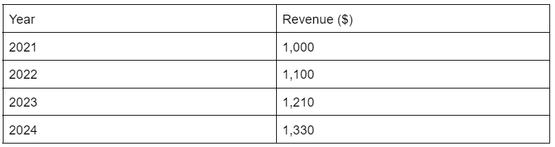
If you’ve gathered data from fiscal 2021 to fiscal 2024 in Excel:

• End Value: The final value at the end of 2024
• Start Value: The starting value at the beginning of 2021
• Number of periods: The total number of periods from 2021-2024 is 3 years

Calculating CAGR in Excel

Here are the steps you can take in Excel:

1. Gather your Start and End Values

• Start Value: $1,000

• End Value: $1,330

2. Calculate the Number of Periods

• Periods are the # of years between the start and end dates.
• So in this case, there are 3 periods between ‘21 and ‘24 (Periods: 2021 -> 2022, 2022 -> 2023, 2023 -> 2024).

3. Plug in the values to our CAGR formula

• CAGR = (1,330 / 1,000)^(1/3) – 1

4. Enter the formula in Excel

• Assuming start year is A2, start value is B2, end year is A5, and end value is B5, then below is the formula we can use.
• =(B5/B2)^(1/YEAR(A5)-YEAR(A2)) – 1

5. Format the result as a percentage

• Format the cell with the CAGR result as a percentage, which gives us a 9.97% CAGR.

With this, you can take historical data and calculate the annualized CAGR growth rate in Excel. The key is structuring your data properly and using the correct CAGR formula.

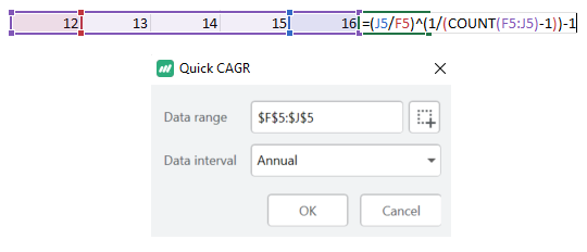
Quick CAGR Excel Shortcut using Macabacus

Calculating CAGR can be calculated easily using the Macabacus add-in for Excel.

Macabacus can quickly insert compound annual growth rate (CAGR) formulas, so you don’t have to remember the formula or manually count periods. 

1. Select a cell to insert the CAGR calculation.
2. Click the Macabacus > Formulas > Quick CAGR  button.
3. Macabacus will intelligently determine which cells to include (left or above) by analyzing surrounding data.
   a. In addition to an annual CAGR, you can easily compute quarterly and monthly growth rates.

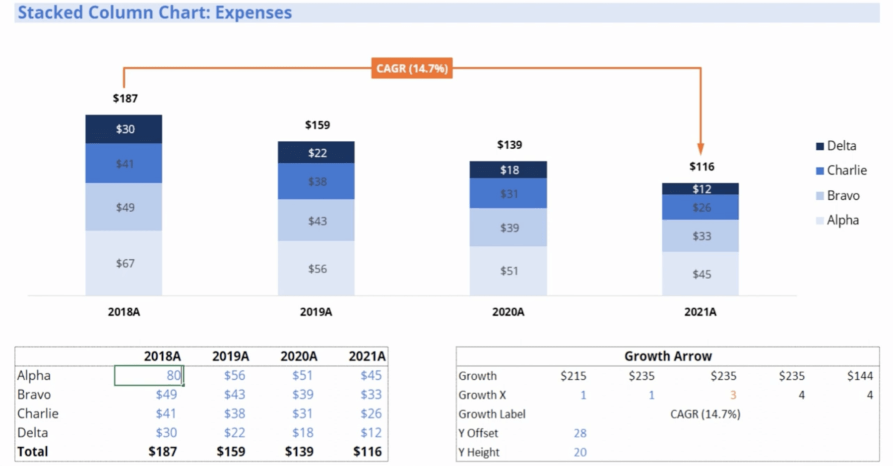
Adding CAGR to an Excel Column Chart with Macabacus

Video Tutorial #1

Video Tutorial #2

Adding a CAGR growth arrow is a great way to visualize growth trends in your Excel charts. With Macabacus, inserting a dynamic CAGR arrow only takes a few clicks.

1. Select the Chart

To start, click on the chart in your workbook where you want to place the CAGR arrow. 

2. Click the Growth Arrow Button

In the Macabacus ribbon, go to: Charts > Growth Arrow

Alternatively, use the keyboard shortcut (Ctrl + Shift + R)

This will insert a default CAGR arrow on the chart.

3. Customize the Arrow

Now you can customize the arrow’s style, color, trajectory, and data label.

Under Growth Arrow Options, tweak items like:

• Arrow Style: Straight, curved, angled, etc.
• Arrow Color: Match chart colors or customize
• Arrow Weight

4. Set the Arrow’s Position to Dynamic

Under Dynamic Setting, switch on the “Dynamic Arrow” option.

This automatically updates the CAGR arrow when the source data changes. The growth arrow will now reflect your latest CAGR each time the chart updates. No manual adjustments needed.

And that’s it! With these four simple steps, you can add dynamic CAGR growth arrows to any Excel chart using Macabacus.