Step-by-Step: Format Excel Chart Data Labels as Thousands or Millions

When creating Excel charts, it’s easy to encounter issues during the display of large numbers on the value axis. Typically, Excel defaults to a full number format, showcasing all zeros (example: 1,500,000), which can lead to complications. Optimizing the axis for readability by cleanly formatting Excel chart data to millions or thousands can prevent it from appearing crowded and difficult to read.

Turn 1,600,000 -> 1.6M

And 900,000 -> 900K

We’ll dig into how to do this in Excel natively, but if you want a shortcut to handle this formatting in seconds, skip ahead.

The Problem with Large Numbers on Excel Charts

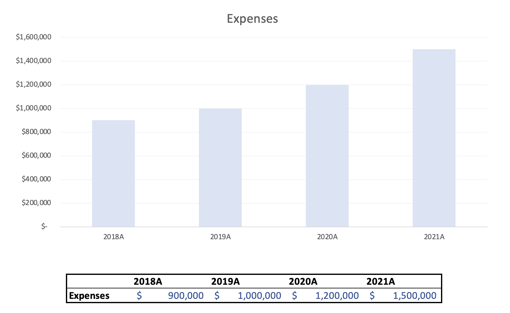
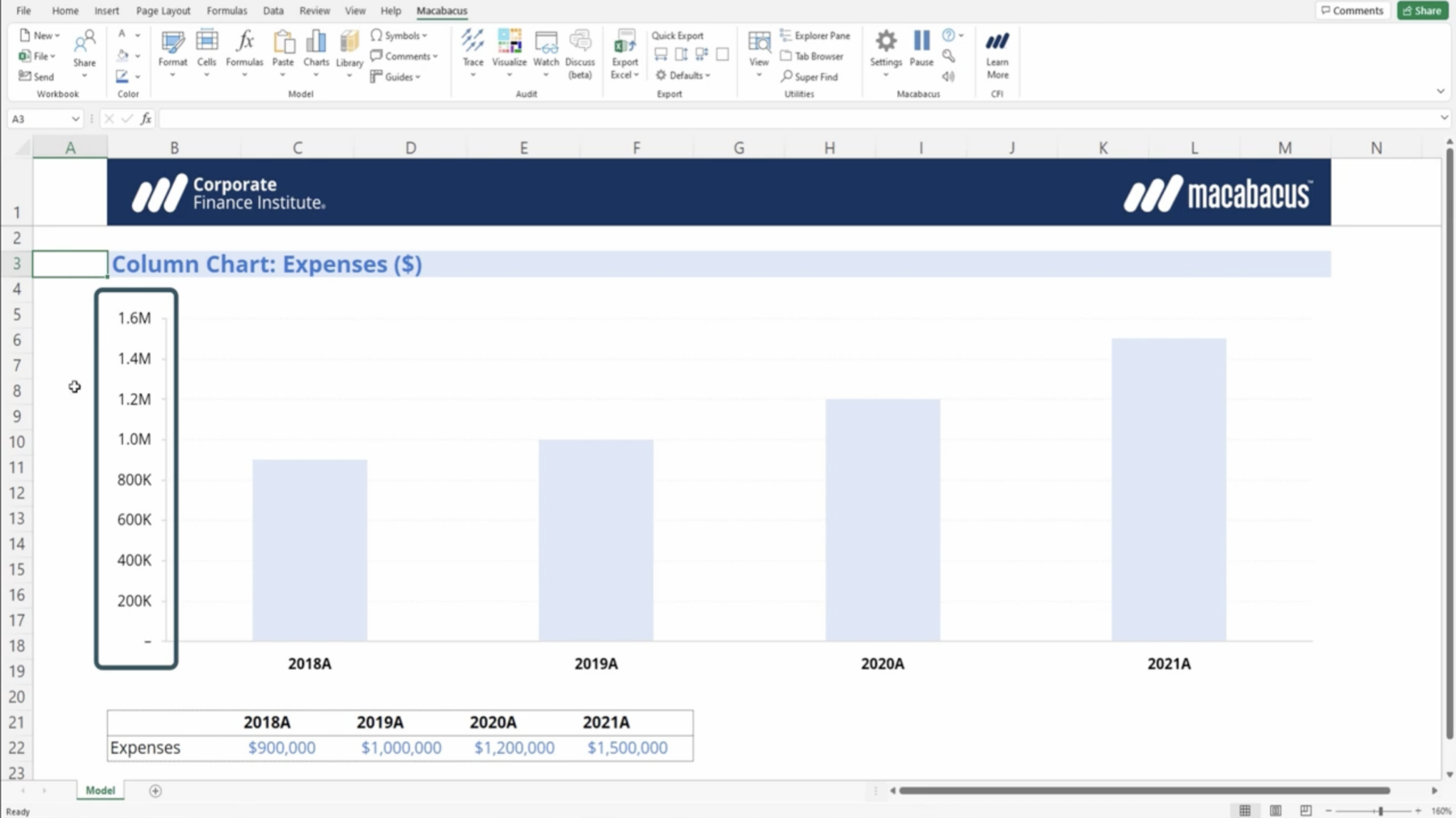
Let’s look at an example. Here’s a column chart showing revenue by year. The amounts range from 0 to 1.6 million.

You can see that the y-axis feels cluttered with all those zeros. It’s not very readable or aesthetically pleasing. The core issue is that Excel displays the full unformatted number on charts by default. This works fine for smaller data sets, but isn’t ideal for larger numbers.

Built-In Options to Format the Value Axis

Luckily, Excel provides a few built-in options to format the value axis units

• Thousands – Displays numbers in thousands (example: 1.6K for 1,600)
• Millions – Displays numbers in millions (example: 1.5M for 1,500,000)
• Billions – Displays numbers in billions (example: 1.5B for 1,500,000,000)

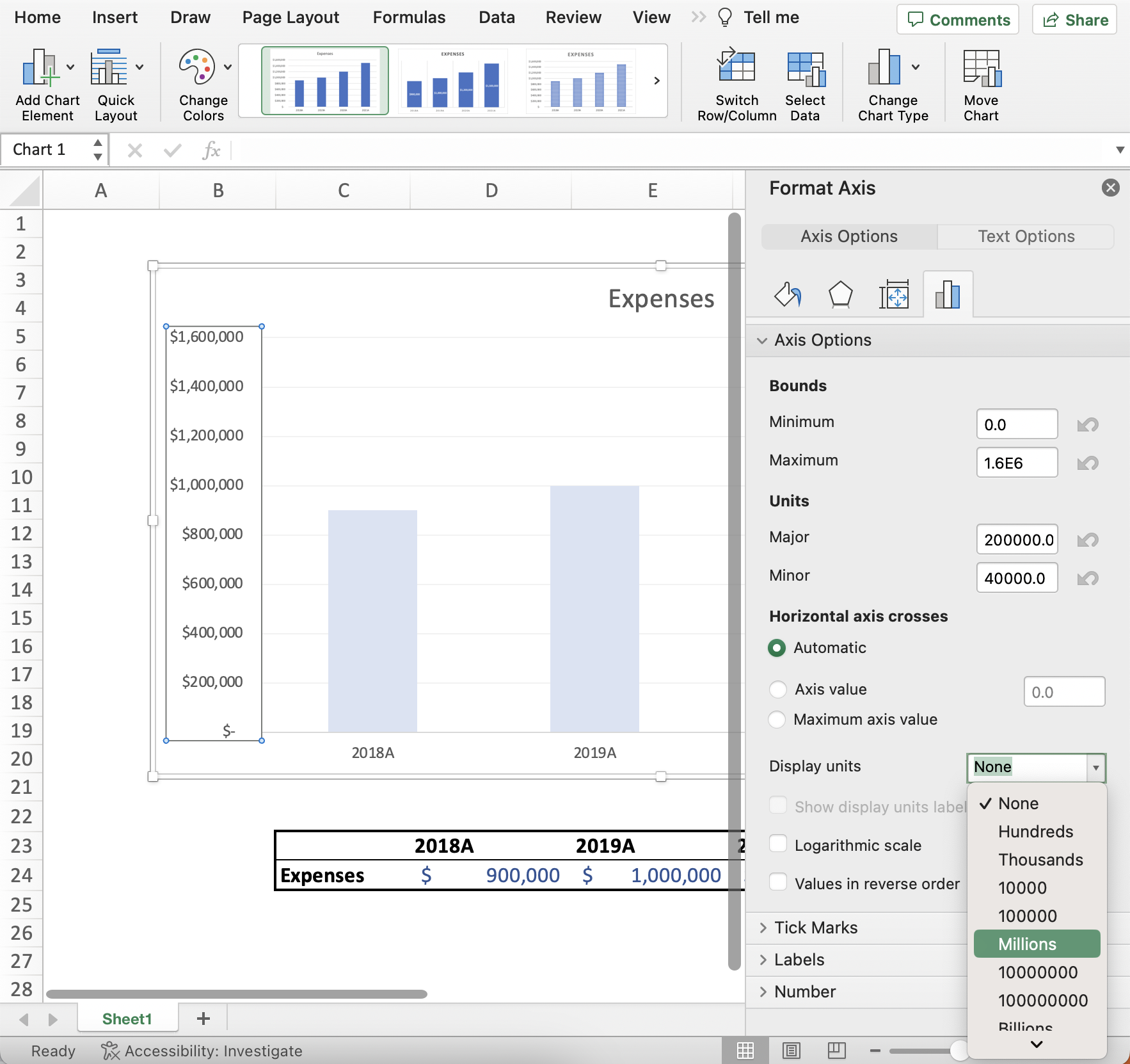
To access these options

1. Select the chart and go to Chart Design > Add Chart Elements > Axes > Primary Vertical
2. In the Format Axis pane, go to Axis Options > Units
3. Choose the desired units: Thousands, Millions, or Billions
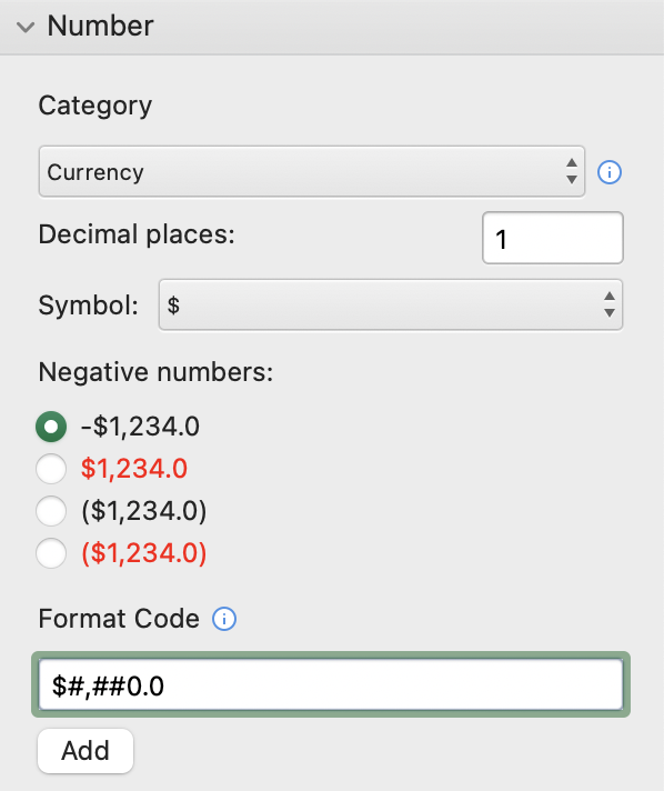
4. Go to the “Number” dropdown and insert: $* #,##0.#_

This will automatically scale the units on the axis and add the appropriate abbreviation (K, M, B) after the numbers.

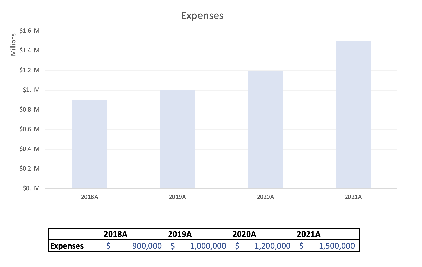
Here’s how the chart looks after formatting to millions:

Much cleaner and easier to read! The axis only displays the necessary units without cluttering it up with extra zeros.

Limitations of Built-In Formatting

The built-in options work well, but you do have a few limitations.

• You will have to manually update the chart if the data changes substantially. Excel doesn’t dynamically recalculate the best scale.
• You can only show units in thousands, millions, or billions. There’s no other way to customize other formats like hundred thousands.
• Custom number formatting can be difficult to figure out and, as you can see, sometimes it adds a “1.”. It’s not a huge deal, but is a bit inconsistent with what we’d like to see.

Alternatives for More Customization

To overcome these limitations, you can create custom number formats for the axis:

Millions and Thousands

$* #,##0.#_, “M”;($* #,##0.#_, “K”)

This displays large numbers in millions and smaller numbers in thousands. No abbreviation is shown if not needed.

This lets you fully customize the units, text, separators, decimals, and more. The advantage of creating custom formats is you get complete control. You can tweak it to fit your specific data and preferences. The only caveat is that you’ll need to manually update it if your data changes drastically. There’s no automatic scaling like the built-in options.

Formatting Excel Chart Axis in a Few Clicks with Macabacus

Manually updating axis formats can be tedious, especially with multiple charts. You see this a lot in finance and banking and it’s where Macabacus can help. Macabacus has a simple option to format your Excel charts to millions or thousands with one click. 

Here’s how it works:

1. Download your Macabacus Free Trial
2. Select your chart and go to Macabacus > Charts
3. Scroll to Other Formats > Y-Axis Formats
4. Choose Format for Millions or Format for Thousands

That’s it! Macabacus instantly applies the appropriate formatting across all your selected charts. It also does the work of updating the format dynamically if your data changes substantially. No more manual tweaking needed.

Try a free 30-day trial of Macabacus to format charts and speed up your Microsoft Office workflows.

Macabacus makes it easy to optimize large numbers on your Excel charts. Whether you have a few charts or hundreds, it helps apply and update value axis formats.

Key Takeaways

Large, unformatted numbers can clutter Excel chart axes. Use these approaches to cleanly format the values in millions, thousands, or custom units.

• Leverage Excel’s built-in options of Thousands, Millions, Billions
• Create custom number formatting for advanced customization
• Use Macabacus to automate formatting across charts, with dynamic updates when data changes

Proper number formats help create more readable, professional charts. Try out these options next time you build charts with large data sets in Excel.